Intro to Causality
1. Correlation vs. Causation
Correlation does not imply causation, for example, there is a correlation between ice cream sales and drowning deaths, but it does not mean that ice cream causes drowning – it’s not likely that people swim while holding an ice cream.
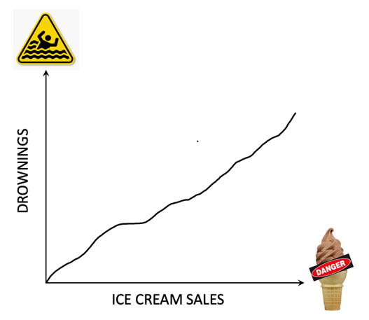

Correlation does not imply causation. But sometimes, it does.
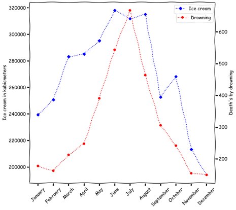
As one plots ice cream sale and drowning deaths over months, it is clear that the correlation between the two is due to the common cause of season. During summer, people buy more ice cream and swim more, leading to more drowning deaths.
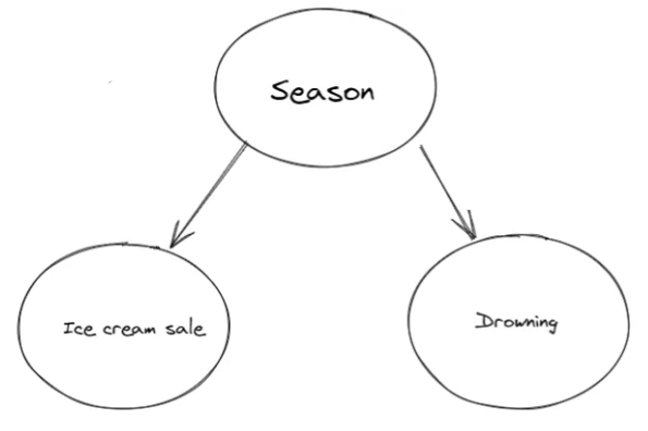
We can represent this relationship with a causal graph, where the season is the common cause of both ice cream sales and drowning deaths. From the graph we can clearly know what is the reason behind the correlation.
2. DAGs
The graph above is an example of a Directed Acyclic Graph (DAG).
A DAG is a graphical representation of causal relationships between variables, consists of nodes and edges, with each edge directed from one node to another (“directed”), such that following those directions will never form a closed loop (“acyclic”).
Directed edges suggest the direction of causality, i.e., $A\rightarrow B$ means $A$ causes $B$.
3. Chains, Forks, and Colliders
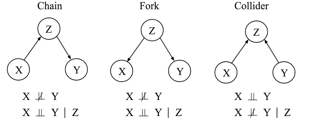
There are three basic structures in DAGs: chains, forks, and colliders.
-
In the case of a chain, $X$ causes ($\rightarrow$) $Z$, and $Z$ causes ($\rightarrow$) $Y$. In a chain model, $X$ and $Y$ are not independent ($X\dep Y$) without conditioning on $Z$. For example, consider three standing dominoes in order $X$, $Z$, and $Y$. The falling of $X$ will cause $Z$ to fall, which in turn will cause $Y$ to fall. However, when we condition on $Z$, the other two variables, $X$ and $Y$, will be independent ($X\indep Y \mid Z$). In other words, if we let domino $Z$ fall, the subsequent domino $Y$ will fall regardless of whether the prior domino $X$ fell or not.
-
In the case of a fork, a single variable $Z$, called a confounder, causally influences two other variables $X$ and $Y$. For instance, consider the influence of rainy weather ($Z$) on both umbrella sales ($X$) and the number of people jogging outside ($Y$). On rainy days, more umbrellas are likely to be sold, and less people will go out for a jog. In a fork model, without conditioning on the confounder $Z$, the other variables, $X$ and $Y$, will be dependent on each other ($X\dep Y$). If one were to analyze umbrella sales and jogging activity without considering the weather, they will find them to be dependent. However, once we condition on the confounder $Z$ and compare days with the same weather condition, umbrella sales and jogging activity should be independent of each other ($X\indep Y \mid Z$).
-
A collider refers to the case that two variables, $X$ and $Y$, independently cause a third variable $Z$. Consider the tossing of two fair coins $X$ and $Y$, and a bell $Z$ that rings whenever both coins lands on heads (this example is still valid when $Z$ is a bell that rings whenever at least one of the coins lands on heads). Without revealing if the bell rings or not, the head/tail states of two coins are independent to each other ($X\indep Y$)—simply as how coin tosses naturally works. However, if we condition on the bell $Z$ not ringing, knowing one of the coins landed on heads immediately informs us that the other coin landed on tails ($X\dep Y \mid Z$), otherwise the bell would have rung.
Note that chains and forks share the same (conditional) independencies, while colliders have a different set of (conditional) independencies. Chains and forks are then considered as the same Markov Equivalence Class (MEC), while colliders belong to a different MEC. Note that these examples operate under the Markov assumption: $X \indep_\textup{Graph} Y \mid Z \Rightarrow X \indep_\textup{Data} Y \mid Z$, meaning that the (conditional) independencies encoded in a causal graph should appear in its data.(Here, we are referring to the global Markov assumption, which is implied by the local Markov assumption. The local Markov assumption states that given its parents in a DAG, a node $X$ is independent of all its non-descendants.)
4. Composite Causal Structures
In cases with more than three variables, variables can potentially be connected through multiple paths, with several chains, forks, or colliders. Following the (conditional) independencies encoded by chains, forks, and colliders, a path is blocked when conditioning on the middle variable of a chain or a fork and unblocked when not conditioning on the middle variable of a chain or a fork. Furthermore, a path is blocked when not conditioning on the middle variable of a collider and unblocked when conditioning on the middle variable of a collider. Two variables are defined to be d-separated if every path between them is blocked. Thus, d-separated variables are independent.

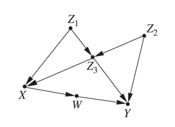
In the DAG below, one will find $Z_2 \dep X$ without any conditioning, since there is an unblocked chain path $Z_2 \rightarrow Z_3 \rightarrow X$.\
One should also find $Z_2 \indep X \mid (Z_3,Z_1)$. Conditioning on $Z_3$ blocks the $Z_2 \rightarrow Z_3 \rightarrow X$ chain. Over the $Z_2 \rightarrow Z_3 \leftarrow Z_1 \rightarrow X$ path, although conditioning on $Z_3$ unblocks the $Z_2 \rightarrow Z_3 \leftarrow Z_2$ collider, the conditioning on $Z_1$ blocks the $Z_3 \leftarrow Z_1 \rightarrow X$ fork, making this path blocked. The remaining $Z_2 \rightarrow Y \leftarrow W \leftarrow X$ path is blocked by the collider $Z_2 \rightarrow Y \leftarrow W$ without conditioning on $Y$.\
Similarly, $Z_2 \dep X \mid (Z_3,Z_1,Y)$.
5. Causal Discovery
5.1.Intervention
When one observes a correlation between two variables, he might make a hypothesis about the causation, or formulate a model using domain knowledge and intuition.
The model might reproduce the observed correlation, but it might not be the true model, as different models can produce the same correlation – for example, Ptolemy’s epicycles and Copernicus’s heliocentrism both predict the same planetary motion.
To nail down the true model, one needs to perform interventions, such as randomized controlled trials. For example, the drug trial is a common intervention in medical studies, where the drug is given to one group and a placebo to another group, and the outcomes are compared.
Intervention is the gold standard to determine causation.
5.2. Causal Discovery from Observational Data
However, in many cases, interventions are impossible, unethical, or impractical. For example, one cannot randomly shut down half of all galaxies’ AGN feedback in the universe to study the effect of AGN feedback on galaxy evolution.
In such cases, the field of causal discovery comes into play, which aims to infer causal relationships from observational data.
5.2.1. Constraint-based Methods
Constraint-based methods infer causal relationships by examining the conditional independencies between variables, since different MECs encode distinct conditional independencies. (Here, we adopt the faithfulness assumption, or the converse of the Markov assumption: $X \indep_\textup{Data} Y \mid Z \Rightarrow X \indep_\textup{Graph} Y \mid Z$.)
A commonly used constraint-based method is the PC (Peter-Clark) algorithm. The PC algorithm consists of three steps:
- Start with a fully-connected, undirected graph among all variables, and remove edges based on conditional independence tests to arrive at a graph skeleton.
- Identify colliders with conditional independence tests and orient them.
- Orient edges that are incident on colliders such that no new colliders will be constructed.
Here is an example of running PC, showing how it goes from a skeleton to a oriented DAG.:

Note that in addition to the Markov assumption and faithfulness assumption, the PC algorithm further assumes causal sufficiency (i.e., no unobserved confounders) and acyclicity.
Another constraint-based method, the FCI (Fast Causal Inference) algorithm relaxes the assumption of causal sufficiency, allowing unobserved confounders. The FCI algorithm is based on the same independence testing procedure as the PC algorithm but differs at the stage of labeling and orienting edges.
5.2.2. Score-based Methods
Instead of finding a single causal structure, we can adopt a Bayesian perspective and define a posterior over all possible DAGs, $P(G \mid D)$. To do this, score-based methods assign a numerical score to every DAG given the data. There are several possible ways to define such a score, such as the Bayesian Information Criterion (BIC) score, generalized score, and the Bayesian Gaussian equivalent (BGe) score, the Bayesian Dirichlet equivalent (BDe) score.
In an exact posterior approach, one evaluates the chosen score for every possible DAG, i.e., $P(G \mid D)$. However, the cost of an exact search grows super-exponentially as the number of variables (nodes) increases. Check out the number of possible DAGs/MECs for N nodes here:
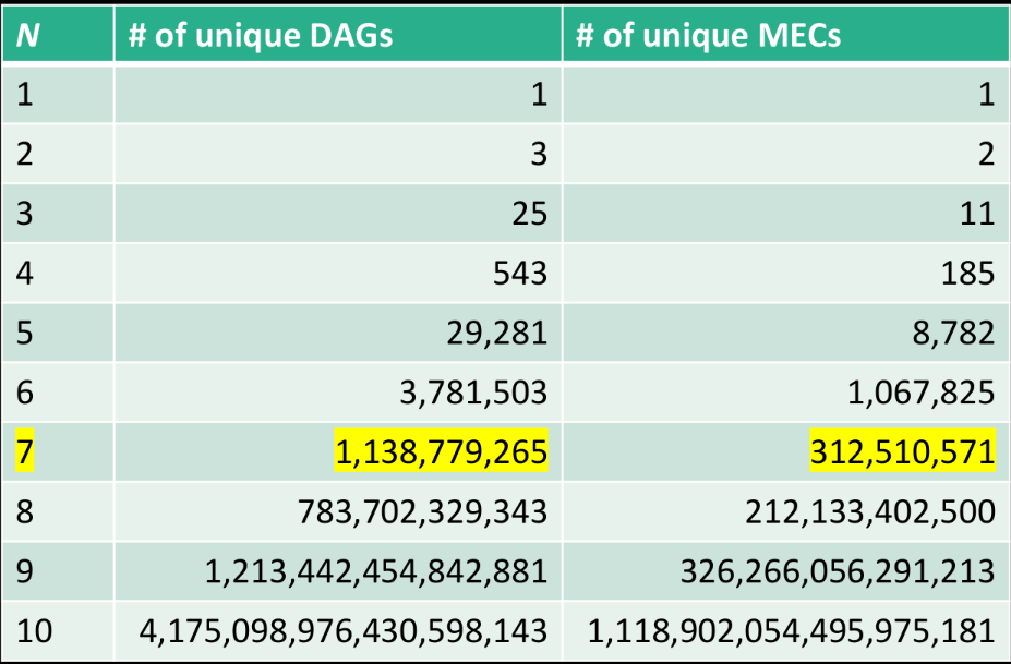
I would not personally recommend an exact search for more than 7 nodes.
As a result, sampling algorithms have been developed to approximate the exact posterior distribution without going over all DAGs. Such approximation is often done with Markov Chain Monte Carlo (MCMC) methods, such as the MC3 algorithm and Gadget.
More recently, neural network based algorithms such as DAG-GFN are also developed to approximate the posterior distribution.
6. Recommended Resources
- Books:
- Causality by Judea Pearl
- Causal inference in statistics : a primer by Judea Pearl, Madelyn Glymour, and Nicholas P. Jewell
- Online Courses:
- Causal discovery Python Libraries:
- Graphical Models Python Libraries: